Analysis of simulated MRWs

The pymultifracs package estimates the multifractal properties of time series. This is an example using simulated Multifractal Random Walks which covers all steps of the multifractal analysis procedure and gives an overview of the toolbox’s features.

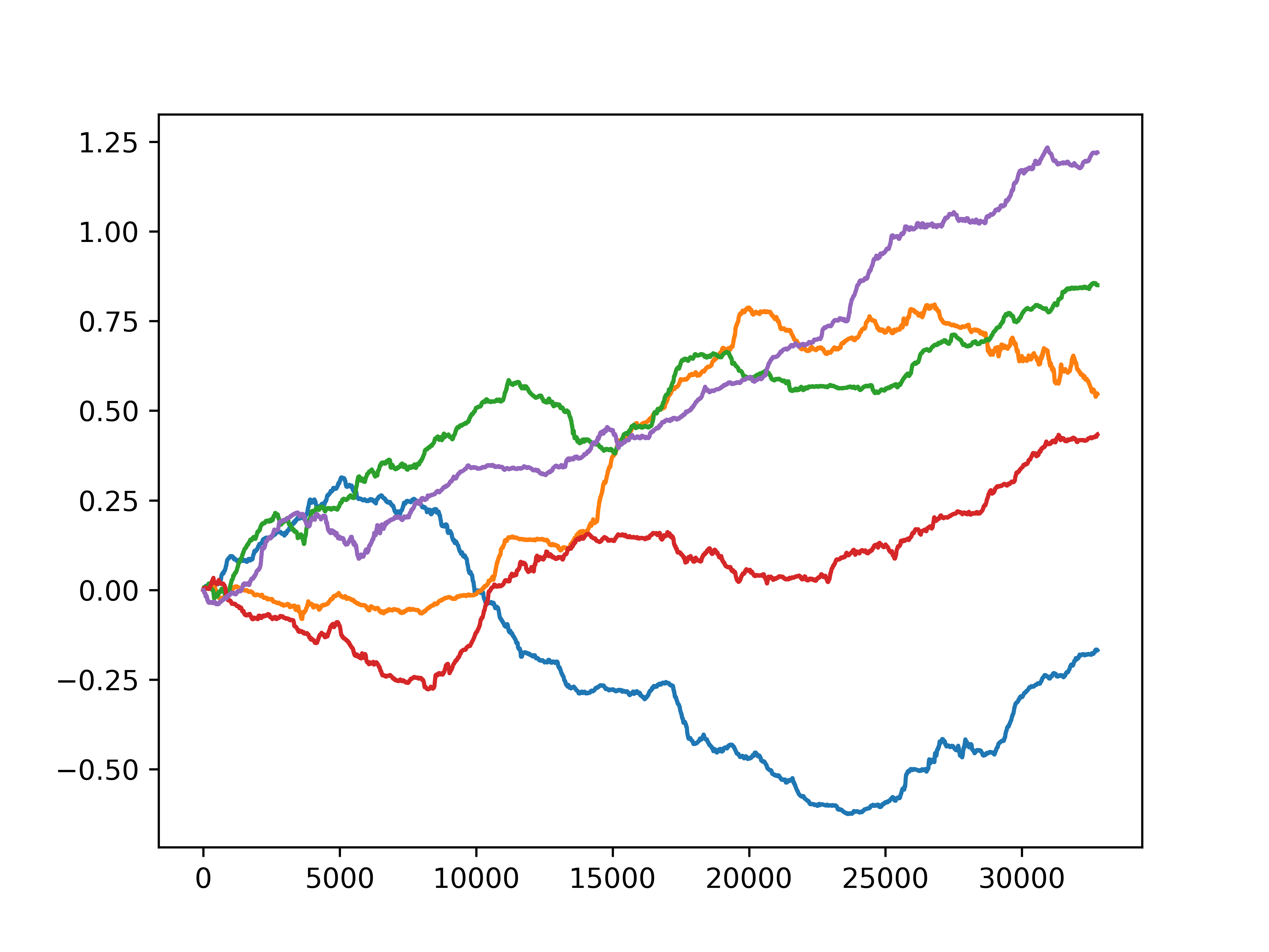
Let us first generate a few Multifractal Random Walks with parameters \(H = 0.8\) and \(\lambda=\sqrt{0.05}\)

import matplotlib.pyplot as plt
import numpy as np
from pymultifracs.simul import mrw

X = mrw(shape=(2**15, 5), H=0.8, lam=np.sqrt(.05), L=2**15)
plt.plot(X)
plt.show()

Wavelet transform

Wavelet transform is performed the pymultifracs.wavelet_analysis() function

Parameters:

• wt_name: The discrete wavelet to use, following the convention of the

pywavelets package.

• j2: The largest scale to analyze, by default None which means that

the analysis is carried to the coarsest possible temporal scale. The motivation for setting a lower value is to reduce the computation time and memory footprint.

• normalization: Normalization norm for the wavelet coefficients: takes

the value of \(p\) to define the \(p\)-norm used in normalization. Defaults to 1 (\(1\)-norm) which is appropriate for scale invariance analysis.

Multivariate time series, such as we are dealing with here, are passed with the shape (n_samples, n_channels)

from pymultifracs import wavelet_analysis

WT = wavelet_analysis(X, wt_name='db3', j2=None, normalization=1)

The output is a WaveletDec object, which contains the wavelet transform of the time series.

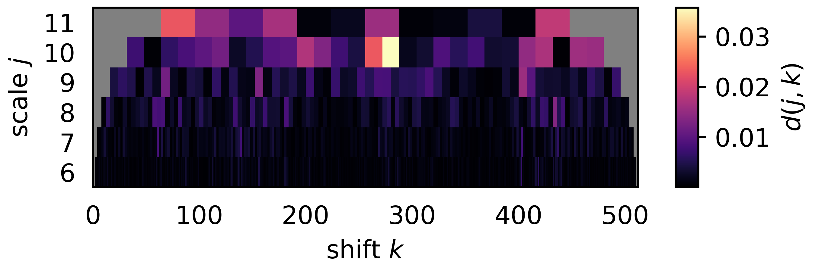
It may be visualized using the plot method, specifying j1 and j2, the lower and upper bounds on the scales temporal scales displayed, respectively.

WT.plot(j1=6, j2=11)

Multi-resolution quantities derived from the wavelet transform can be obtained using the associated methods WaveletDec.get_leaders() and WaveletDec.get_wse():

WTL = WT.get_leaders(p_exp=np.inf)
WTpL = WT.get_leaders(p_exp=2)
WSE = WT.get_wse(theta=0.5)

Multifractal Analysis

Multifractal analysis relies on regressing a linear relationship between the temporal scale \(j\) and statistical quantities that are a function of \(j\). The range of scales over which the regression is performed, usually chosen as the range of scales for which the data is scale-invariant. The scaling_ranges argument is a list of tuples indicating the bounds of the range of scales to use for regression. Multiple scaling ranges may be regressed at once by providing multiple tuples:

scaling_ranges = [(2, 8), (3, 8)]

Minimal regularity

In order for the analysis to be meaningful under the chosen multifractal formalism (wavelet coefficient, wavelet (p-)leader, etc.) it may be necessary to verify a minimum regularity condition. The method WaveletDec.check_regularity() is available with all multi-resolution quantities, and takes scaling_ranges as an argument:

WT.check_regularity(scaling_ranges)
WTL.check_regularity(scaling_ranges)
WTpL.check_regularity(scaling_ranges)
WSE.check_regularity(scaling_ranges)

In case the minimal regularity is too low, it may be necessary to fractionally integrate the time series.

A simple approach is provided in the WaveletDec.auto_integrate() method, which will try to find a fractional integration coefficient large enough that all signals may be analyzed, and return the properly integrated multi-resolution quantity.

WTpL = WTpL.auto_integrate(scaling_ranges)

Otherwise, and for instance in the case where multiple sets of data need to be compared using the same integration coefficient, the fractional integration can be set using the WaveletDec.integrate() method on a MRQ object by passing the fractional integration coefficient \(\gamma\):

WT_int = WT.integrate(.5)

Analysis

Multifractal analysis is carried out using the mfa() function.

Basic parameters:

• mrq: Multi-resolution quantity (WaveletDec,

WaveletLeader, WaveletWSE) on which to perform the analysis.

• weighted: whether the linear regressions should be weighted. Defaults

to None, which means no weighting is performed. "Nj" indicates that the weights are determined from the number of coefficients at each scale.

• q: list of moments.

Note

by default, mfa() checks the regularity of the time series.

It is possible to disable this by passing check_regularity=False.

from pymultifracs import mfa
from pymultifracs.utils import build_q_log

pwt = mfa(WTpL, scaling_ranges, weighted='Nj', q=[-2, -1, 0, 1, 2])

The function outputs a MFractalVar object, which contains:

• structure: the structure functions (StructureFunction) and

associated exponents

• cumulants: the cumulant scaling functions (Cumulants) and

log-cumulants

• spectrum: the multifractal spectrum (MFSpectrum)

Plotting

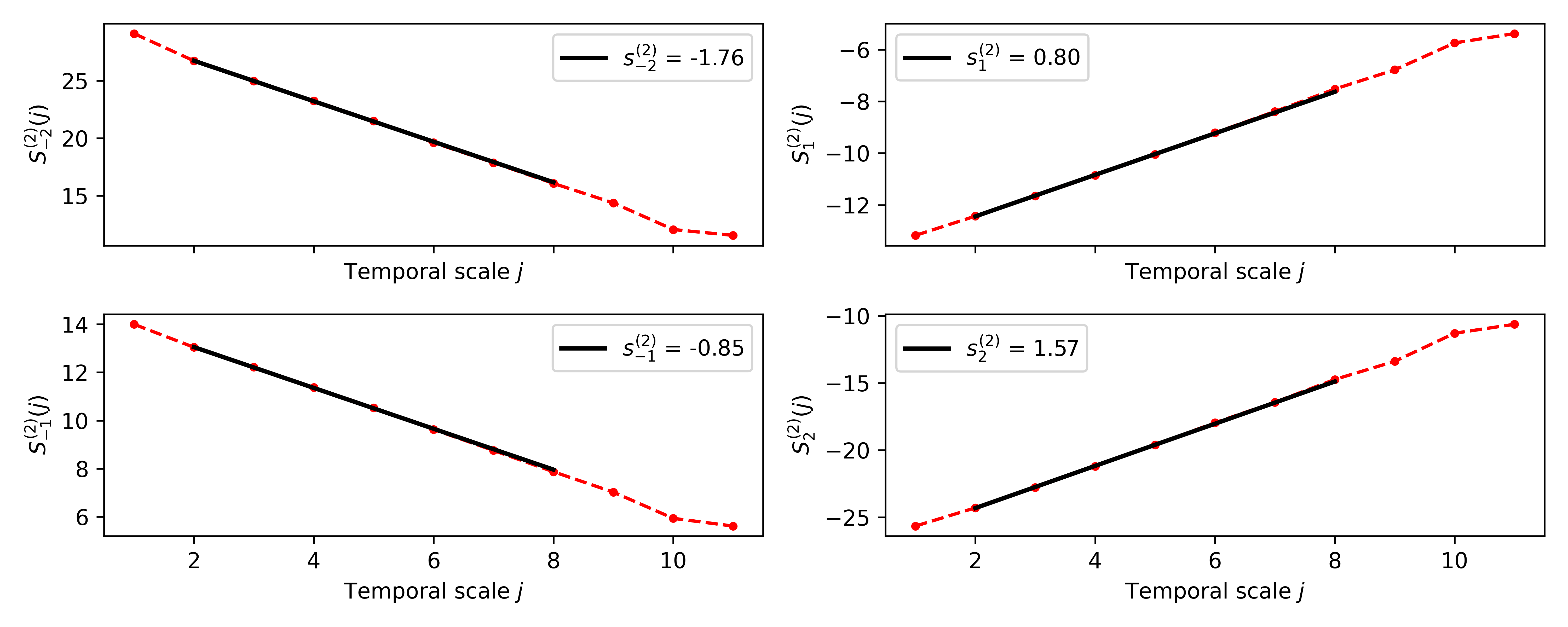
Structure functions

The structure functions \(S_q(j)\) and their associated exponents may be visualized using the StructureFunction.plot() method

pwt.structure.plot(figsize=(10, 4), nrow=2)

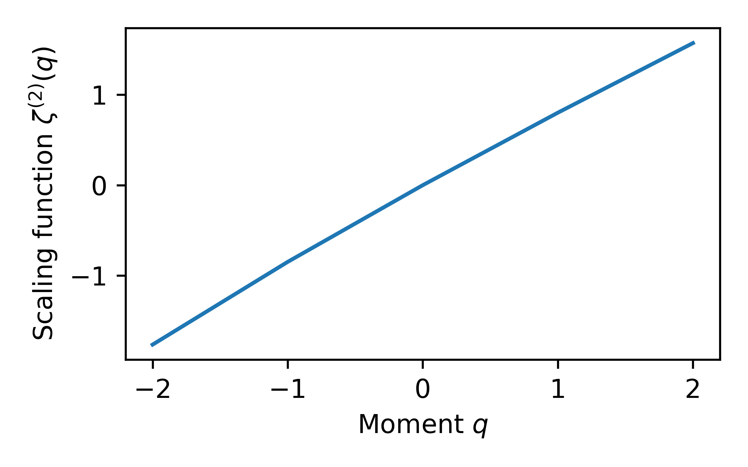
We can plot \(\zeta(q)\) using the StructureFunction.plot_scaling() method

pwt.structure.plot_scaling()

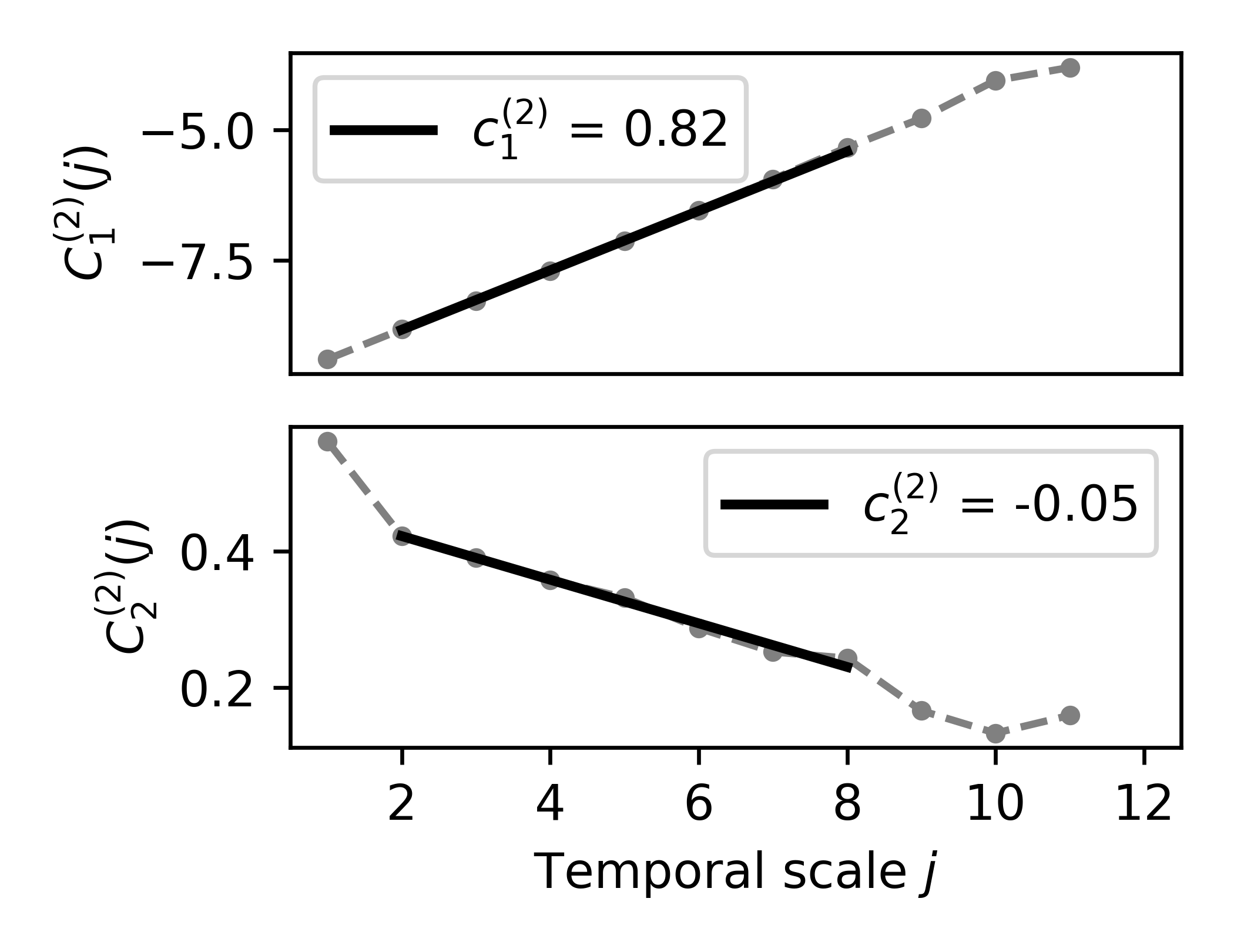
Cumulants

The cumulant scaling functions may be visualized using Cumulants.plot()

pwt.cumulants.plot()

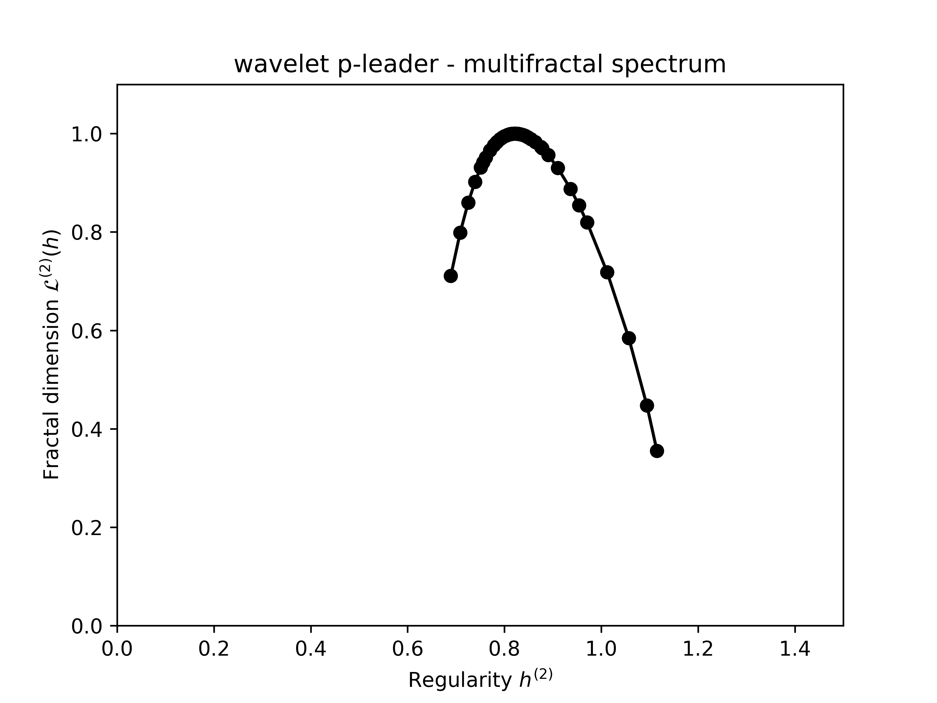
Multifractal spectrum Visualizing the multifractal spectrum requires more densely sampled values of \(q\):

pwt = mfa(WTpL, scaling_ranges, weighted='Nj', q=build_q_log(.1, 5, 20))
pwt.spectrum.plot()