Analysis of bivariate data

The pymultifracs package can perform bivariate multifractal analysis, and produces bivariate cumulants and structure functions. The purpose of bivariate MFA is to determine the relationship between the regularity fluctuations of a pair of time series.

We will be using pre-generated data to serve as an example of bivariate multi-fractal time series. Let us first load the data; those example time series are also found in the tests/data/ folder of the repository on github.

import pooch
from scipy.io import loadmat

url = ('https://github.com/neurospin/pymultifracs/raw/refs/heads/master/tests/'
       'data/DataSet_ssMF.mat')

fname = pooch.retrieve(url=url, known_hash=None, path=pooch.os_cache("bivar"))

X = loadmat(fname)['data'].T

Downloading data from 'https://github.com/neurospin/pymultifracs/raw/refs/heads/master/tests/data/DataSet_ssMF.mat' to file '/home/runner/.cache/bivar/c2970ce816c6ddbf5b2539426c580fc7-DataSet_ssMF.mat'.
SHA256 hash of downloaded file: 7027dfe19282c5802ff5e3bbab2fca7d9fb744c874a853d82883c2b0fed6fb57
Use this value as the 'known_hash' argument of 'pooch.retrieve' to ensure that the file hasn't changed if it is downloaded again in the future.

The data is a two-dimensional array, with both self-similarity and multifractal correlation.

import matplotlib.pyplot as plt

fig, ax = plt.subplots(2, 1, sharex=True)
ax[0].plot(X[:, 0])
ax[1].plot(X[:, 1], c='C1')

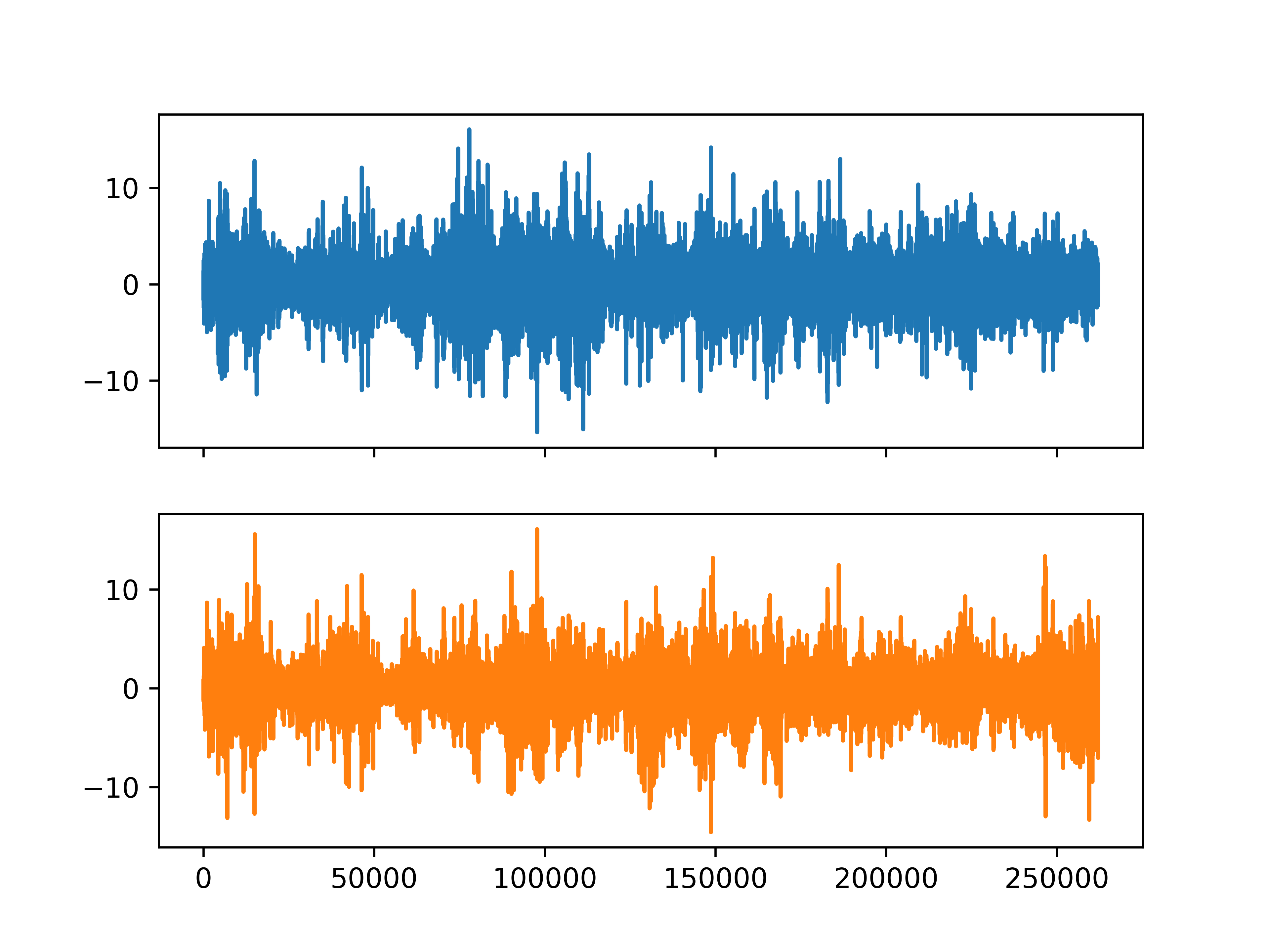
[<matplotlib.lines.Line2D object at 0x7f71df1a87d0>]

First we need wavelet_analysis() as ususal, to obtain p-leaders in this case

from pymultifracs import wavelet_analysis

WTpL = wavelet_analysis(X).integrate(.75).get_leaders(2)

Then we use bivariate.bimfa() on the wavelet p-leaders. We provide the same MRQ twice, in order to compute the estimates for all signal pairs.

import numpy as np
from pymultifracs.bivariate import bimfa

q1 = np.array([0, 1, 2])
q2 = np.array([0, 1, 2])

pwt = bimfa(WTpL, WTpL, scaling_ranges=[(3, 9)], q1=q1, q2=q2)

# We can obtain the multifractal correlation matrix :math:`\rho_{mf}`:

print(pwt.cumulants.rho_mf.squeeze())

<xarray.DataArray (channel1: 2, channel2: 2)> Size: 32B
array([[1.        , 0.71314563],
       [0.71314563, 1.        ]])
Coordinates:
    m1       int64 8B 1
    m2       int64 8B 1
Dimensions without coordinates: channel1, channel2

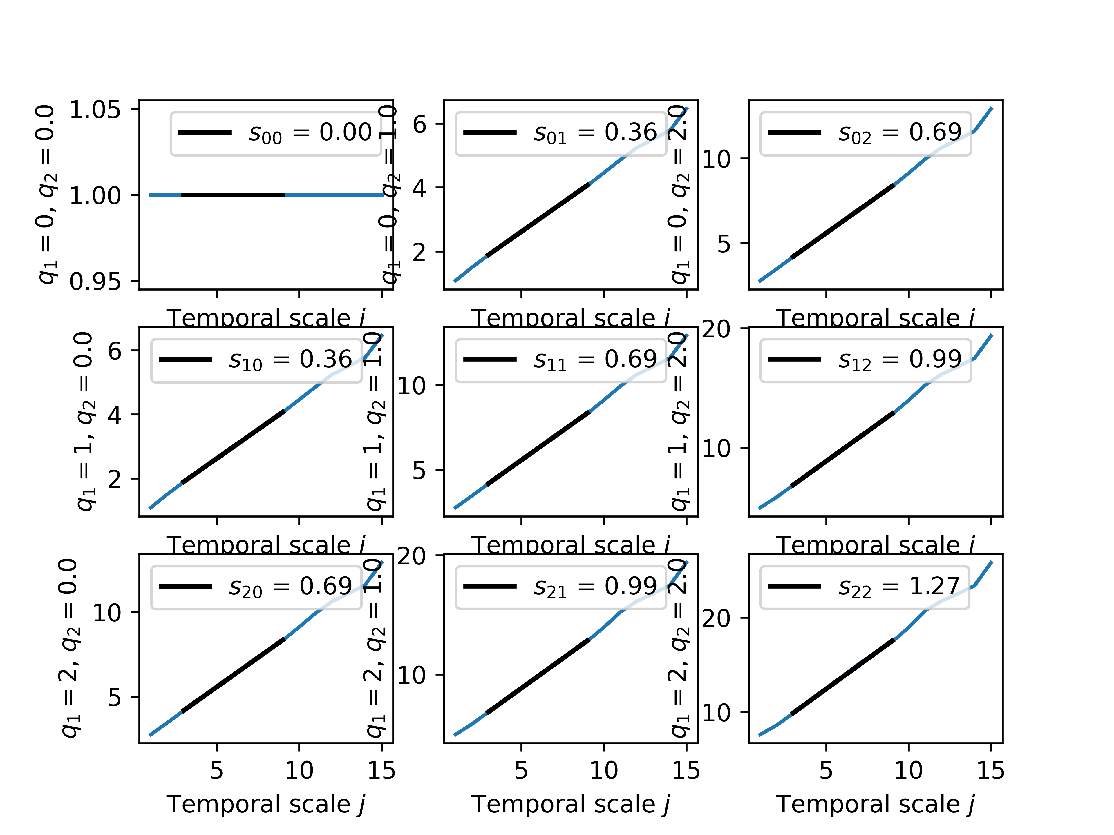
We can plot the structure function:

pwt.structure.plot()

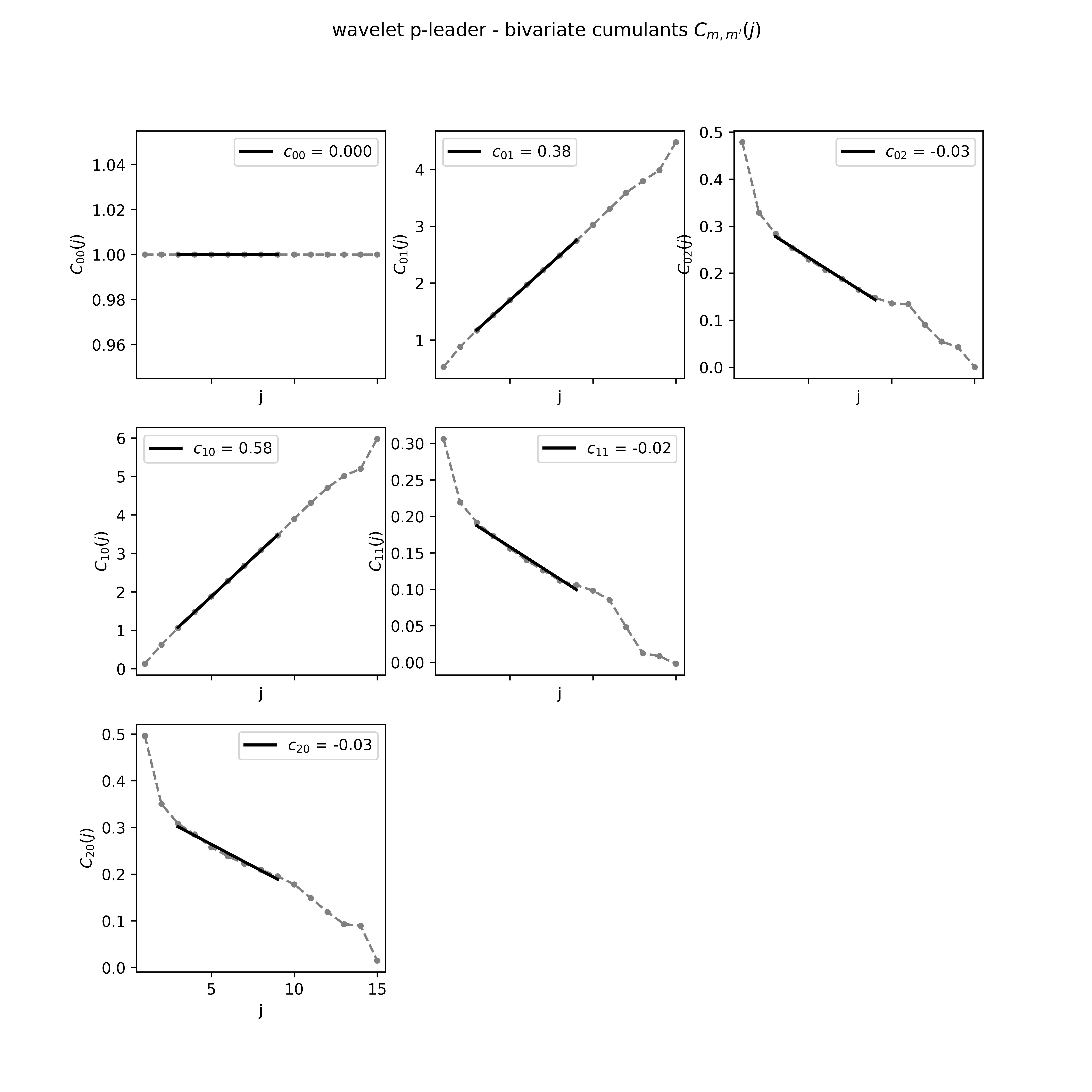
We can plot the bivariate cumulants:

pwt.cumulants.plot()

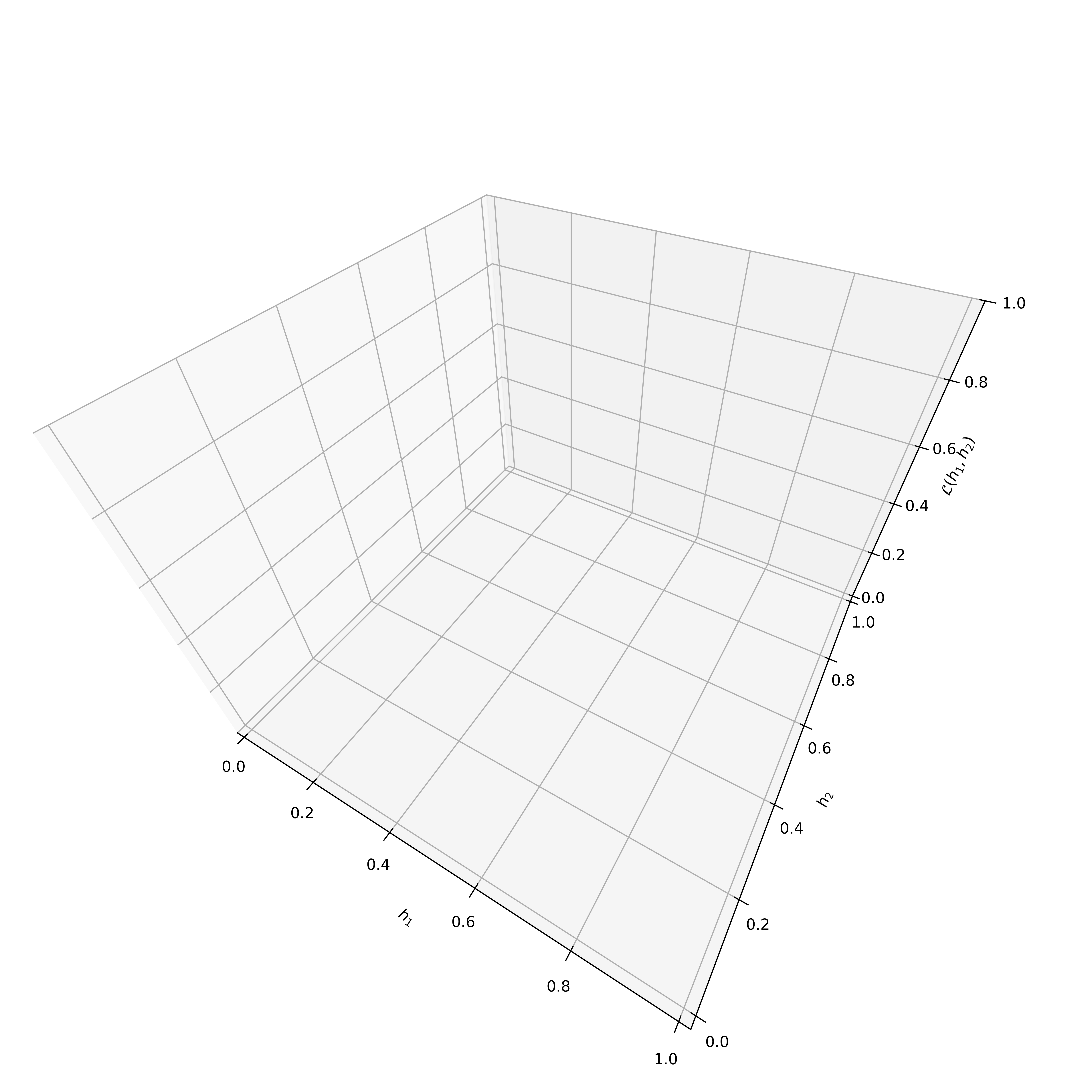
We can plot the Legendre spectrum reconstituted from the log-cumulants:

pwt.cumulants.plot_legendre(h_support=(.1, .95))