Benchmarking estimation methods

The pymultifracs toolbox provides a tool to benchmark different methods for estimating the multifractal exponent, different parameter for those methods on different synthetic scale free time series, with different parameter for those time series.

This is done via the Benchmark class We provide here a simple example for Benchmarking methods.

import numpy as np

from pymultifracs.simul import fbm, mrw
from pymultifracs import wavelet_analysis, mfa
from pymultifracs.robust.benchmark import Benchmark

We must first define the functions generating signals

N = 2 ** 12


def fbm_gen(H):
    return fbm(H=H, shape=(N, 40))


def mrw_gen(H):
    return mrw(H=H, shape=(N, 40), L=N, lam=np.sqrt(.05))

Then we define the signal generation parameter grids:

signal_param_grid = {
    'fbm': {
        'H': np.array([.7, .8])
    },
    'mrw': {
        'H': np.array([.7, .9])
    }
}

signal_gen_grid = {
    'fbm': fbm_gen,
    'mrw': mrw_gen,
}

We then define the functions that will estimate the multifractal analysis paramters.

def pleader_est(X, p_exp):

    WT = wavelet_analysis(X).get_leaders(p_exp=p_exp)
    pwt = mfa(WT, [(3, 7)], estimates='c', weighted='Nj')

    out = pwt.cumulants.log_cumulants.isel(
        scaling_range=0).to_series().unstack('m')
    out.columns = out.columns.to_flat_index().map(lambda x: f'c{x}')

    return out


def coef_est(X):

    WT = wavelet_analysis(X)
    dwt = mfa(WT, [(3, 7)], estimates='c')

    out = dwt.cumulants.log_cumulants.isel(
        scaling_range=0).to_series().unstack('m')
    out.columns = out.columns.to_flat_index().map(lambda x: f'c{x}')

    return out

This is completed by defining the parameter grids, similarly to how it was done for the signal generating functions.

estimation_param_grid = {
    'pleader': {
        'p_exp': np.array([0.5, 1, 2, 5]),
        },
    'coef': {}
}
estimation_grid = {
    'pleader': pleader_est,
    'coef': coef_est,
}

Finally, we instantiate the Benchmark class and compute the benchmark.

bench = Benchmark(
    signal_gen_grid, signal_param_grid, estimation_grid, estimation_param_grid)
bench.compute_benchmark()

  0%|          | 0/4 [00:00<?, ?it/s]
 25%|██▌       | 1/4 [00:00<00:02,  1.43it/s]
 50%|█████     | 2/4 [00:01<00:01,  1.41it/s]
 75%|███████▌  | 3/4 [00:02<00:00,  1.26it/s]
100%|██████████| 4/4 [00:03<00:00,  1.24it/s]
100%|██████████| 4/4 [00:03<00:00,  1.28it/s]

We obtain results in the form of a dataframe, which contains all combinations of signal model and signal parameters, and analysis method and method parameters.

bench.results.query('method=="pleader"').head(10)

				m	c1	c2
model	H	method	p_exp	channel
fbm	0.7	pleader	0.5	0	0.689874	-0.021826
				1	0.622390	-0.019494
				2	0.666206	-0.036636
				3	0.644672	-0.022084
				4	0.710006	-0.023396
				5	0.630358	-0.018044
				6	0.702269	-0.020622
				7	0.667735	-0.022948
				8	0.728175	-0.024603
				9	0.739451	-0.021211

We can then derive statistics from that dataframe.

bench.results.xs(
    ('fbm', 'pleader', .7), level=('model', 'method', 'H')
    ).groupby('p_exp').mean()

m	c1	c2
p_exp
0.5	0.681789	-0.024059
1.0	0.682994	-0.015227
2.0	0.683818	-0.005799
5.0	0.683197	0.001009

Seaborn can effectively use the results dataframe to show group statistics. For instance, comparing the performance of the wavelet p-leader estimation is a one-line command:

import seaborn as sns

sns.boxplot(data=bench.results.xs(
    ('mrw','pleader'), level=('model', 'method')), x='p_exp', y='c2')

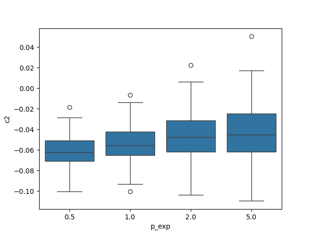
<Axes: xlabel='p_exp', ylabel='c2'>